
Constructing and Interpreting Acceleration-Time Graphs
Acceleration-time graphs provide a visual representation of the rate of change of velocity of an object over time. Understanding these graphs is fundamental in kinematics.
Creating Acceleration-Time Graphs
- Time Axis: The horizontal axis of the graph represents time, typically in seconds (s).
- Acceleration Axis: The vertical axis denotes acceleration, usually in meters per second squared (m/s²).
- Plotting Data: Points are plotted on the graph based on the acceleration at different time intervals.

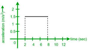
Acceleration-time graph
Image Courtesy Science Facts
Interpreting Different Graph Features
- Horizontal Lines: A horizontal line indicates constant acceleration. The height of the line from the time axis shows the magnitude of this constant acceleration.
Constant acceleration in acceleration-time graph
Image Courtesy GeeksforGeeks
- Sloping Lines: A sloping line suggests that acceleration is changing over time. An upward slope indicates increasing acceleration, while a downward slope shows decreasing acceleration.
- Positive and Negative Values: Points above the time axis represent positive acceleration, while those below indicate negative acceleration, often interpreted as deceleration.
Gradient and Area Analysis in Acceleration-Time Graphs
The gradient and area under the curve in acceleration-time graphs hold significant information about the motion of an object.
Understanding Gradient
- Gradient Calculation: The gradient of a line on an acceleration-time graph is determined by dividing the change in acceleration by the change in time.
- Significance of Gradient: In a graph with a straight line, the gradient is constant, indicating uniform acceleration. In contrast, a changing gradient on a curved line points to non-uniform acceleration.
Area Under the Graph
- Area Calculation: The area under an acceleration-time graph is found by calculating the integral of the acceleration with respect to time.
- Relevance of Area: This area represents the change in velocity of the object over the specified time period.
Distinguishing Between Constant and Variable Acceleration
Understanding the distinction between constant and variable acceleration is crucial in interpreting acceleration-time graphs.
Characteristics of Constant Acceleration Graphs
- Representation: A graph depicting constant acceleration features a straight horizontal line.
- Implications: The object experiences the same rate of acceleration throughout the time interval.
Identifying Variable Acceleration
- Graph Characteristics: Variable acceleration is represented by a non-linear graph. The line may be curved or have different slopes at different intervals.
- Understanding Variable Acceleration: The rate of acceleration is changing throughout the motion. This could be due to various factors like external forces or changes in the object's environment.
Practical Applications and Examples
Acceleration-time graphs are not merely theoretical; they find applications in various fields, providing insights into different motion scenarios.
Real-World Examples
- Transportation: Analyzing the acceleration graphs of vehicles helps in understanding their performance and efficiency.
- Sport Science: Athletes' performances, particularly in sprinting and cycling, can be analysed through acceleration graphs to improve training regimes.
Problem-Solving with Graphs
Acceleration-time graphs are valuable in problem-solving scenarios, such as:
- Calculating Change in Velocity: By determining the area under the graph, one can calculate how much an object’s velocity has changed over a period.
- Understanding Motion: These graphs provide a visual understanding of how objects speed up, slow down, or maintain a steady speed.
FAQ
The area under an acceleration-time graph represents a change in velocity because acceleration is defined as the rate of change of velocity. When we calculate the area under this graph, we are essentially integrating acceleration with respect to time. Integration of acceleration (a change in velocity per unit time) over time gives us the total change in velocity. This is different from distance, which is the integral of velocity with respect to time. Thus, the area under an acceleration-time graph gives us how much the velocity of an object has changed over a certain time period, not the distance it has travelled.
Uniform circular motion on an acceleration-time graph can be identified by a constant, non-zero acceleration value. This is because, in uniform circular motion, the speed of the object remains constant, but its direction (and hence velocity) is continually changing, resulting in a constant centripetal acceleration towards the centre of the circle. This constant acceleration is reflected as a straight, horizontal line on the acceleration-time graph that does not intersect the time axis. The line's position above or below the time axis indicates the direction of acceleration, but its constant nature signifies the uniformity of the circular motion.
Yes, acceleration-time graphs can have negative areas, and they hold significant meaning. A negative area occurs when the acceleration-time graph lies below the time axis, indicating negative acceleration or deceleration. This negative area signifies a decrease in the velocity of the object over the time interval considered. For example, if a car is slowing down, the acceleration-time graph will dip below the time axis, and the area enclosed between the graph and the axis will be negative, representing the reduction in the car's velocity. This concept is crucial in understanding braking mechanisms or any scenario where objects decelerate.
In an acceleration-time graph, positive and negative acceleration are distinguished by the position of the graph line in relation to the time axis. Positive acceleration is represented by parts of the graph that lie above the time axis. This indicates that the object's velocity is increasing over time. Negative acceleration, or deceleration, is depicted by portions of the graph that are below the time axis. This shows that the object's velocity is decreasing over time. The key is the graph's position relative to the horizontal time axis – above for positive acceleration and below for negative acceleration.
An acceleration-time graph is a powerful tool for analysing vehicle performance. It illustrates how quickly a vehicle can change its speed, which is vital for understanding its capability in situations like overtaking or emergency braking. For instance, a steep slope on the graph indicates rapid acceleration, which is desirable in performance vehicles. Conversely, a gradual slope signifies slower acceleration, common in heavier vehicles or those with less powerful engines. Additionally, the graph can also show the effectiveness of braking systems through the deceleration phase, where negative acceleration values are plotted. By studying these graphs, engineers and drivers can assess and compare the performance characteristics of different vehicles.
Practice Questions
To find the total change in velocity, we calculate the area under the acceleration-time graph. The graph forms a trapezium with two parts: a triangle for the first 5 seconds and a rectangle for the next 5 seconds. The area of the triangle is 1/2 * base * height = 1/2 * 5 s * 10 m/s² = 25 m/s. The area of the rectangle is base * height = 5 s * 10 m/s² = 50 m/s. Adding these together, the total change in velocity over the 10 seconds is 25 m/s + 50 m/s = 75 m/s.
The average acceleration can be determined by calculating the slope of the acceleration-time graph. The graph shows a straight line with a negative slope going from 4 m/s² to -4 m/s² over 4 seconds. The change in acceleration (Δa) is -4 m/s² - 4 m/s² = -8 m/s². The change in time (Δt) is 4 seconds. Therefore, the average acceleration (a_avg) is Δa / Δt = -8 m/s² / 4 s = -2 m/s². This means the object's average acceleration over the 4-second period is -2 m/s², indicating a deceleration.
