The concept of the Average Rate of Change (ARC) is foundational in calculus, enabling us to understand how one quantity changes in relation to another over a given interval. This calculation divides the change in one variable by the change in another, offering a quantifiable measure of change between two points. Through calculus, the ARC concept evolves, especially as we approach intervals where the change in the independent variable tends toward zero, presenting challenges in traditional calculations.

Understanding Average Rate of Change

Definition: The ARC between two points on a function $y = f(x)$ is defined as:

$ARC = \frac{\Delta y}{\Delta x} = \frac{f(x_2) - f(x_1)}{x_2 - x_1}$

where $\Delta y$ is the change in the function's value, and $\Delta x$ is the change in the independent variable's value.

Importance: This concept is crucial for understanding how the output of a function changes relative to changes in the input, providing a basis for more complex calculus concepts, including the derivative.

Transitioning to Calculus

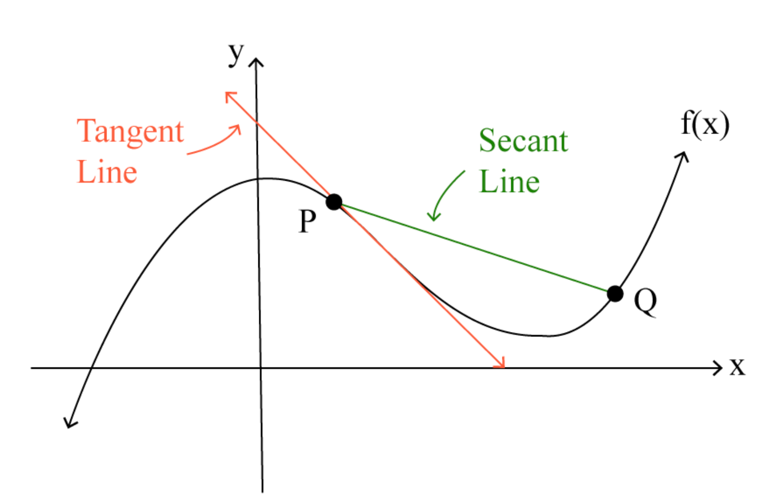
• Limits and the ARC: As the interval $\Delta x$ approaches zero, we encounter the concept of a limit. Calculus allows us to explore what happens to the ARC as $x_2$ approaches $x_1$, moving towards an instantaneous rate of change.

  • Example of applying limits to ARC:

$\lim_{\Delta x \rightarrow 0} \frac{f(x_1 + \Delta x) - f(x_1)}{\Delta x}$

Calculating Average Rate of Change: Examples

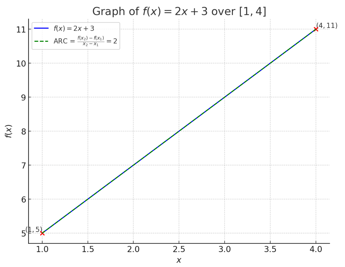
Example 1: Linear Function

Consider the function $f(x) = 2x + 3$ over the interval [1, 4].

• Step 1: Identify $x_1$ and $x_2$, $x_1 = 1$, $x_2 = 4$.

• Step 2: Calculate $f(x_1)$ and $f(x_2)$, $f(1) = 5$, $f(4) = 11$.

• Step 3: Compute ARC,

$\begin{gathered} &&&&& ARC = \frac{f(x_2) - f(x_1)}{x_2 - x_1} \\ &&&&& = \frac{11 - 5}{4 - 1} \\ &&&&& = \frac{6}{3} \\ &&&&& = 2 \end{gathered}$

• Result: The ARC of $f(x)$ over [1, 4] is 2.

• Graphical Representation

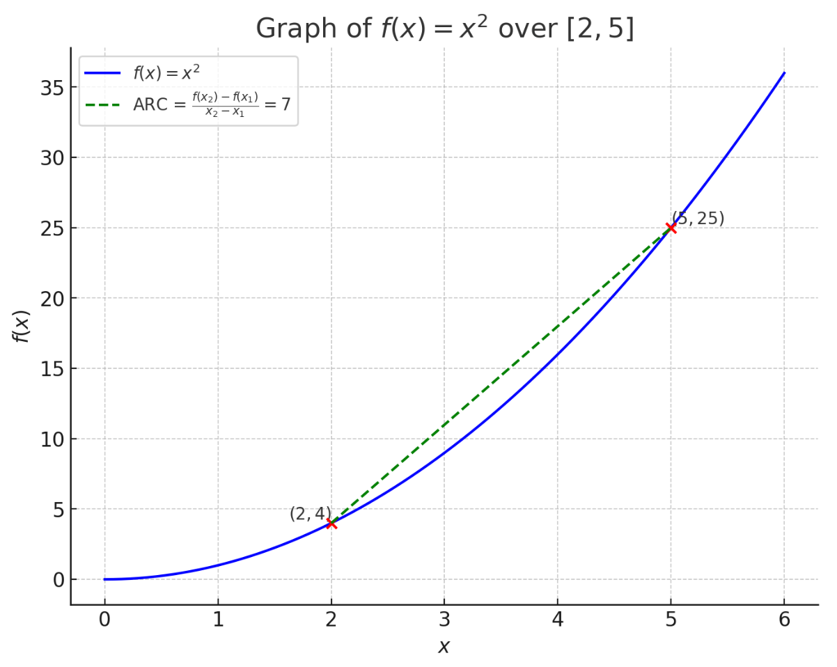
Example 2: Quadratic Function

Consider $f(x) = x^2$ over the interval [2, 5].

• Step 1: Identify points, $x_1 = 2$, $x_2 = 5$.

• Step 2: Evaluate $f(x_1)$ and $f(x_2)$, $f(2) = 4$, $f(5) = 25$.

• Step 3: Calculate ARC,

$\begin{gathered} &&&&& ARC = \frac{f(x_2) - f(x_1)}{x_2 - x_1} \\ &&&&& = \frac{25 - 4}{5 - 2} \\ &&&&& = \frac{21}{3} \\ &&&&& = 7 \end{gathered}$

• Result: The ARC of $f(x)$ over [2, 5] is 7.

• Graphical Representation:

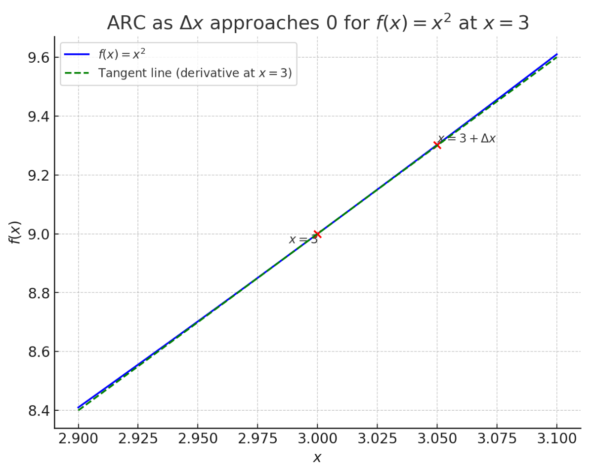
Example 3: Using Limits to Explore ARC's Approach to Zero

Consider $f(x) = x^2$ as $\Delta x$ approaches 0 from [3, $3 + \Delta x$].

• Step 1: Express ARC as a limit,

$\begin{aligned} && & \lim{\Delta x \rightarrow 0} \frac{f(3 + \Delta x) - f(3)}{\Delta x} \\ && = & \lim{\Delta x \rightarrow 0} \frac{(3 + \Delta x)^2 - 9}{\Delta x} \\ && = & \lim{\Delta x \rightarrow 0} \frac{9 + 6\Delta x + \Delta x^2 - 9}{\Delta x} \\ && = & \lim{\Delta x \rightarrow 0} \frac{6\Delta x + \Delta x^2}{\Delta x} \\ && = & \lim_{\Delta x \rightarrow 0} 6 + \Delta x \\ && = & 6 \end{aligned}$

• Result: As $\Delta x$ approaches 0, the Average Rate of Change of $f(x) = x^2$ at $x = 3$ approaches 6. This reflects the instantaneous rate of change, or derivative, of $f(x)$ at $x = 3$.

• Graphical Representation:

Example 4: Real-World Application

Consider a vehicle's distance traveled, described by $f(t) = 4t^2 + 2t$ where $f(t)$ is distance in meters and (t) is time in seconds, over the interval [1, 4] seconds.

• Step 1: Identify $t_1 = 1$, $t_2 = 4$.

• Step 2: Calculate $f(t_1)$ and $f(t_2)$, $f(1) = 6$, $f(4) = 72$.

• Step 3: Compute ARC,

$\begin{aligned} && ARC = \frac{f(t_2) - f(t_1)}{t_2 - t_1} \\ && = \frac{72 - 6}{4 - 1} \\ && = \frac{66}{3} \\ && = 22 \end{aligned}$

• Result: The vehicle's average speed over the interval [1, 4] seconds is 22 meters per second.

Example 5: Changing Rates

For a balloon being inflated, the volume $V$ in cubic centimeters is given by $V(t) = \frac{4}{3}\pi(6t)^3$ where $t$ is time in minutes. Calculate the ARC of volume change between 2 and 5 minutes.

• Step 1: Identify $t_1 = 2$, $t_2 = 5$.

• Step 2: Calculate $V(t_1)$ and $V(t_2)$,

$\begin{aligned} &&&&& V(2) & = \frac{4}{3}\pi(6 \cdot 2)^3, \\ &&&&& V(5) & = \frac{4}{3}\pi(6 \cdot 5)^3. \end{aligned}$

• Step 3: Compute ARC,

$\begin{aligned} ARC & = \frac{V(t_2) - V(t_1)}{t_2 - t_1} \\ & = \frac{\frac{4}{3}\pi(6 \cdot 5)^3 - \frac{4}{3}\pi(6 \cdot 2)^3}{5 - 2} \\ & = \frac{4}{3}\pi \left( \frac{(6 \cdot 5)^3 - (6 \cdot 2)^3}{3} \right) \\ & = 468\pi \end{aligned}$

• Result: The average rate of volume change between 2 and 5 minutes is $468\pi$ cubic centimeters per minute, illustrating how volumes of three-dimensional shapes can change over time.

Practice Questions

Question 1

Given the function $f(x) = 3x^2 - 2x + 5$, calculate the average rate of change from $x = 1$ to $x = 4$.

Question 2

A spherical balloon is being inflated so that its volume at any time $t$ in seconds is given by $V(t) = \frac{4}{3}\pi t^3$. Calculate the average rate of change of the balloon's volume from $t = 2$ seconds to $t = 5$ seconds.

Question 3

For the function $g(x) = \ln(x)$, compute the average rate of change between $x = 1$ and $x = e$, where $e$ is the base of natural logarithms.

Solutions to Practice Questions

Solution to Question 1

1. Identify the function and points: $f(x) = 3x^2 - 2x + 5, x_1 = 1, x_2 = 4$.

2. Calculate $f(x_1)$ and $f(x_2)$:

$f(1) = 3(1)^2 - 2(1) + 5 = 6, \\ f(4) = 3(4)^2 - 2(4) + 5 = 41.$

3. Compute the average rate of change:

$\begin{aligned} ARC &= \frac{f(x_2) - f(x_1)}{x_2 - x_1} \\ &= \frac{41 - 6}{4 - 1} \\ &= \frac{35}{3} \\ &= 11\frac{2}{3}. \end{aligned}$

4. Result: The average rate of change from $x = 1$ to $x = 4$ is $11\frac{2}{3}$.

Solution to Question 2

1. Given volume function: $V(t) = \frac{4}{3}\pi t^3$, with $t_1 = 2$ and $t_2 = 5$.

2. Find $V(t_1)$ and $V(t_2)$:

$V(2) = \frac{4}{3}\pi (2)^3 = \frac{32}{3}\pi, \\ V(5) = \frac{4}{3}\pi (5)^3 = \frac{500}{3}\pi.$

3. Calculate ARC:

$\begin{aligned} ARC &= \frac{V(t_2) - V(t_1)}{t_2 - t_1} \\ &= \frac{\frac{500}{3}\pi - \frac{32}{3}\pi}{5 - 2} \\ &= \frac{468\pi}{3} \\ &= 156\pi. \end{aligned}$

4. Result: The average rate of change of the volume from $t = 2$ to $t = 5$seconds is $156\pi$ cubic units per second.

Solution to Question 3

1. Identify the function and interval: $g(x) = \ln(x)$, from $x = 1$ to $x = e$.

2. Calculate $g(x_1)$ and $g(x_2)$:

$g(1) = \ln(1) = 0, \\ g(e) = \ln(e) = 1.$

3. Compute the ARC:

$\begin{aligned} ARC &= \frac{g(x_2) - g(x_1)}{x_2 - x_1} \\ &= \frac{1 - 0}{e - 1} \\ &= \frac{1}{e - 1}. \end{aligned}$

4. Result: The average rate of change of $g(x)$ between $x = 1$ and $x = e$ is $\frac{1}{e - 1}$.

Velocity is the first derivative of position: $( v_x = \frac{dx}{dt} )$

Average acceleration: The total change in velocity divided by the total time taken:

$a=ΔvΔta = \frac{\Delta v}{\Delta t}a=ΔtΔv​$

Understanding Kinematics

Kinematics is a branch of physics that deals with the mathematical description of motion. Unlike dynamics, which explores the causes of motion through forces, kinematics focuses solely on the geometric aspects of movement. This fundamental approach allows us to develop a strong foundation in motion analysis before introducing the complexities of forces and their interactions.

The Language of Motion

Basic Motion Concepts

• Motion occurs when an object's position changes relative to a reference point over time

• The study of kinematics requires defining a coordinate system with clear directionality

• One-dimensional motion involves movement along a single axis, typically denoted as the x-axis

• All motion can be described using three fundamental quantities: position, velocity, and acceleration

• The relationships between these quantities form the basis of kinematic analysis

Reference Frames

• A reference frame provides the essential context for describing motion

• It consists of:

  • An origin point (0,0) from which all measurements are taken

  • A clearly defined positive direction

  • A coordinate system with appropriate units

  • A time measurement system

• The choice of reference frame affects our mathematical description of motion but not the physical motion itself

• Multiple reference frames can describe the same motion differently, yet all are equally valid

Vector Quantities in One Dimension

Position Vector

• Position $(x)$ represents an object's location relative to the origin at a specific time

• In one dimension, position is represented by a single coordinate along the chosen axis

• The SI unit for position is the meter (m)

• Position can be:

  • Positive: indicating location in the positive direction from origin

  • Negative: indicating location in the negative direction from origin

  • Zero: indicating location at the origin

• Expressed mathematically as:

  • $\vec{x} = x\hat{i}$ where $\hat{i}$ is the unit vector in the x-direction

• The change in position, or displacement, is given by:

  • $\Delta x = x_f - x_i$

Velocity Vector

Understanding Velocity

• Velocity describes the rate of change of position with respect to time

• It includes both speed (magnitude) and direction (sign in one dimension)

• The SI unit is meters per second (m/s)

• Velocity is mathematically represented as:

  • $\vec{v} = \frac{d\vec{x}}{dt}$

• The instantaneous velocity vector points in the direction of motion at any given moment

Types of Velocity

• Instantaneous velocity: velocity at a specific moment in time

  • Defined as the limit of average velocity as time interval approaches zero

  • $v = \lim_{\Delta t \to 0} \frac{\Delta x}{\Delta t}$

• Average velocity: total displacement divided by total time interval

  • $\vec{v}_{avg} = \frac{\Delta \vec{x}}{\Delta t} = \frac{x_f - x_i}{t_f - t_i}$

• The sign of velocity indicates direction in one dimension:

  • Positive velocity: motion in positive direction

  • Negative velocity: motion in negative direction

  • Zero velocity: momentary rest or direction change

Acceleration Vector

Defining Acceleration

• Acceleration represents the rate of change of velocity with respect to time

• Describes how quickly velocity changes in magnitude and/or direction

• SI unit is meters per second squared (m/s²)

• Mathematical expression:

  • $\vec{a} = \frac{d\vec{v}}{dt}$

• Average acceleration can be calculated as:

  • $\vec{a}_{avg} = \frac{\Delta \vec{v}}{\Delta t} = \frac{v_f - v_i}{t_f - t_i}$

Important Acceleration Concepts

• Can be positive or negative, independent of velocity

• Constant acceleration: acceleration remains unchanged over time

  • Common in many physical situations

  • Simplifies mathematical analysis

• Variable acceleration: acceleration changes with time

  • Requires calculus for complete analysis

  • More common in real-world situations

• Acceleration occurs when:

  • Speed changes (speeding up or slowing down)

  • Direction changes (in higher dimensions)

  • Both speed and direction change simultaneously

Sign Conventions in One Dimension

Understanding Signs

• Signs (+/-) indicate direction along the chosen axis

• Positive direction: typically right or up, depending on axis orientation

• Negative direction: typically left or down

• Consistent sign conventions are crucial for accurate problem-solving

• Signs help track:

  • Direction of motion

  • Changes in direction

  • Relative motion between objects

Vector Nature in One Dimension

• Although one-dimensional motion occurs along a single axis, quantities remain vectors

• Direction is indicated by:

  • Sign of the quantity (+ or -)

  • Unit vector notation ($\hat{i}$)

• Vector addition and subtraction follow algebraic rules in one dimension

• The dot product simplifies to regular multiplication in one dimension

Applications in Real-World Scenarios

Examples of One-Dimensional Motion

• Vertical motion of a thrown ball

• Cars moving along a straight highway

• Elevator moving up and down

• Objects falling under gravity

• Train moving along straight tracks

• Rocket launch (initial vertical ascent)

Common Misconceptions

• Speed versus velocity

  • Speed is scalar (magnitude only)

  • Velocity is vector (magnitude and direction)

• Position versus displacement

  • Position is absolute location

  • Displacement is change in position

• Average versus instantaneous quantities

  • Average describes overall behavior

  • Instantaneous describes behavior at a specific moment

• The significance of positive and negative values

  • Signs indicate direction, not magnitude

  • Negative acceleration doesn't always mean slowing down

Remember that kinematics provides the mathematical framework needed to describe motion, forming the basis for more advanced concepts in mechanics. Understanding these foundational concepts is crucial for success in AP Physics C: Mechanics.

Kinematics forms the foundation of mechanics, focusing on describing and analyzing motion through mathematical relationships, without considering the underlying forces that cause the motion.

Introduction to Kinematics: Understanding Motion

The Nature of Kinematics

Kinematics is the branch of physics that describes the motion of objects through space and time, without considering the forces that cause the motion. This fundamental area of physics provides the mathematical tools and concepts needed to analyze movement and make predictions about an object's future position and velocity.

Understanding kinematics is crucial because it:

• Forms the foundation for studying more complex physics concepts

• Provides essential tools for engineering and design

• Helps explain everyday phenomena

• Develops critical analytical and problem-solving skills

Vector Quantities in One-Dimensional Motion

Position

Position is a vector quantity that describes an object's location relative to a chosen reference point (origin). In one-dimensional motion:

• Denoted by $x$ or $s$ in equations

• Measured in meters (m) in SI units

• Can be positive or negative, indicating direction relative to the origin

• Represented mathematically as: $\vec{x} = x\hat{i}$

• Displacement ($\Delta x$) represents change in position: $\Delta x = x_f - x_i$

Position in Context

When describing position:

• The reference point (origin) must be clearly defined

• Direction from the origin must be specified

• Units must be consistent throughout calculations

• Changes in position consider both magnitude and direction

Velocity

Velocity represents the rate of change of position with respect to time and includes both speed and direction. Velocity is characterized by:

Average Velocity

• Calculated over a finite time interval

• Mathematical expression: $\vec{v}_{avg} = \frac{\Delta x}{\Delta t} = \frac{x_f - x_i}{t_f - t_i}$

• Represents the overall motion during a time period

• May not reflect instantaneous conditions

Instantaneous Velocity

• Describes motion at a specific moment

• Mathematically expressed as: $\vec{v} = \lim_{\Delta t \to 0} \frac{\Delta x}{\Delta t} = \frac{dx}{dt}$

• More useful for analyzing continuous motion

• Can vary from moment to moment

Velocity Characteristics

• SI unit is meters per second (m/s)

• Vector representation: $\vec{v} = v_x\hat{i}$

• Sign indicates direction of motion

• Magnitude equals speed in one dimension

Acceleration

Acceleration is the rate of change of velocity with respect to time. It describes how velocity changes and has several important aspects:

Types of Acceleration

1. Average Acceleration:

   • Calculated over a time interval

   • Mathematical expression: $\vec{a}_{avg} = \frac{\Delta v}{\Delta t} = \frac{v_f - v_i}{t_f - t_i}$

   • Useful for overall motion analysis

2. Instantaneous Acceleration:

   • At a specific moment in time

   • Mathematical expression: $\vec{a} = \lim_{\Delta t \to 0} \frac{\Delta v}{\Delta t} = \frac{dv}{dt}$

   • Critical for detailed motion analysis

Acceleration Properties

• SI unit is meters per second squared (m/s²)

• Vector representation: $\vec{a} = a_x\hat{i}$

• Can be positive, negative, or zero

• Sign indicates direction of velocity change

Vector Nature in One Dimension

Understanding Vectors vs. Scalars

In one-dimensional motion, vector quantities have distinct characteristics:

• Direction indicated by positive or negative signs

• Magnitude represents the size of the quantity

• Vector addition follows algebraic rules: $\vec{A} + \vec{B} = (A_x + B_x)\hat{i}$

• Vector subtraction: $\vec{A} - \vec{B} = (A_x - B_x)\hat{i}$

Reference Frames

The choice of reference frame is crucial in kinematics:

• Defines positive and negative directions

• Establishes the origin (x = 0)

• Must remain consistent throughout problem-solving

• Can affect the mathematical description of motion

Reference Frame Considerations

• Should be chosen to simplify problem-solving

• Must be clearly specified and maintained

• Can be relative to moving or stationary objects

• Affects numerical values but not physical reality

Mathematical Foundations

Calculus Relationships

The fundamental relationships between position, velocity, and acceleration are interconnected through calculus:

Derivative Relationships

• Velocity from position: $v_x = \frac{dx}{dt}$

• Acceleration from velocity: $a_x = \frac{dv_x}{dt}$

• Acceleration from position: $a_x = \frac{d^2x}{dt^2}$

Integration Relationships

• Position from velocity: $x = \int v_x dt$

• Velocity from acceleration: $v_x = \int a_x dt$

• These relationships are crucial for advanced problem-solving

Sign Conventions

Understanding sign conventions is essential for problem-solving:

• Positive direction: Usually right or up

• Negative direction: Usually left or down

• Combined effects:

  • Positive velocity and positive acceleration: Speeding up in positive direction

  • Positive velocity and negative acceleration: Slowing down in positive direction

  • Negative velocity and positive acceleration: Slowing down in negative direction

  • Negative velocity and negative acceleration: Speeding up in negative direction

1.1.1 Introduction to Kinematics

Kinematics is a branch of physics that studies the motion of objects without considering the forces causing the motion. This foundational concept forms the basis for understanding one-dimensional motion and introduces key vector quantities such as position, velocity, and acceleration.

Kinematics: The Study of Motion Without Forces

Kinematics focuses solely on describing how objects move, leaving out the causes of motion, such as forces and energy. It provides a mathematical framework to study motion using equations, graphs, and other tools. By isolating motion from external influences, kinematics enables students to develop a clear understanding of movement in a simplified context.

Key Features of Kinematics

• Focus on motion: Emphasizes movement without analyzing forces.

• Simplified models: Assumes idealized conditions, such as no air resistance.

• Foundation for dynamics: Serves as a prerequisite for studying Newton’s laws.

Understanding Motion in One Dimension

One-dimensional motion occurs when an object moves along a straight line. The motion can either be in a single direction or involve changes in direction along the same line. In kinematics, this is analyzed using three critical vector quantities: position, velocity, and acceleration.

Introduction to Vector Quantities

Vector quantities in kinematics describe motion using both magnitude and direction. These include position (xxx), velocity (vvv), and acceleration (aaa). Understanding these vectors is essential for analyzing one-dimensional motion.

Position (xxx)

Position specifies the location of an object relative to a reference point, often chosen as the origin of a coordinate system.

• Represented as x(t)x(t)x(t), where ttt is time.

• Can have positive or negative values depending on the direction relative to the origin.

• Measured in meters (m) in the SI system.

Example:

An object located 5 m to the right of the origin has x=+5 mx = +5 \, \text{m}x=+5m. If it moves 3 m to the left, its position becomes x=+2 mx = +2 \, \text{m}x=+2m.

Velocity (vvv)

Velocity describes the rate of change of position over time, including the direction of motion. It is calculated using the formula:

v=ΔxΔtv = \frac{\Delta x}{\Delta t}v=ΔtΔx​

Where:

• vvv = velocity (m/s)

• Δx\Delta xΔx = change in position

• Δt\Delta tΔt = change in time

Key Points:

• Instantaneous velocity: The velocity of an object at a specific instant, calculated as: v=dxdtv = \frac{dx}{dt}v=dtdx​

• Average velocity: The total displacement divided by the total time taken: vavg=xfinal−xinitialtfinal−tinitialv_{\text{avg}} = \frac{x_{\text{final}} - x_{\text{initial}}}{t_{\text{final}} - t_{\text{initial}}}vavg​=tfinal​−tinitial​xfinal​−xinitial​​

• Velocity includes direction. A positive velocity indicates motion in the positive direction, while a negative velocity indicates motion in the opposite direction.

Example:

If a car moves 100 m east in 5 seconds, its velocity is:

v=100 m5 s=20 m/sv = \frac{100 \, \text{m}}{5 \, \text{s}} = 20 \, \text{m/s}v=5s100m​=20m/s

If the car reverses and travels 50 m west in 2 seconds, its velocity is:

v=−50 m2 s=−25 m/sv = \frac{-50 \, \text{m}}{2 \, \text{s}} = -25 \, \text{m/s}v=2s−50m​=−25m/s

Acceleration (aaa)

Acceleration measures the rate at which velocity changes over time. It is calculated as:

a=ΔvΔta = \frac{\Delta v}{\Delta t}a=ΔtΔv​

Where:

• aaa = acceleration (m/s²)

• Δv\Delta vΔv = change in velocity

• Δt\Delta tΔt = change in time

Key Points:

• Instantaneous acceleration: The acceleration at a specific moment in time: a=dvdta = \frac{dv}{dt}a=dtdv​

• Average acceleration: The total change in velocity divided by the total time taken: aavg=vfinal−vinitialtfinal−tinitiala_{\text{avg}} = \frac{v_{\text{final}} - v_{\text{initial}}}{t_{\text{final}} - t_{\text{initial}}}aavg​=tfinal​−tinitial​vfinal​−vinitial​​

• Acceleration is a vector quantity. A positive acceleration indicates an increase in velocity in the positive direction, while a negative acceleration (deceleration) signifies a decrease.

Example:

If a car’s velocity changes from 10 m/s10 \, \text{m/s}10m/s to 30 m/s30 \, $\text{m/s}30m/s in 5 seconds, its acceleration is:</p><p>$a=30 m/s−10 m/s5 s=4 m/s2a = \frac{30 \, \text{m/s} - 10 \, \text{m/s}}{5 \, \text{s}} = 4 \, \text{m/s}^2a=5s30m/s−10m/s​=4m/s2</p><hr><h2 id="relationships-between-position-velocity-and-acceleration">Relationships Between Position, Velocity, and Acceleration</h2><p>In one-dimensional motion, these vector quantities are interrelated:</p><ul><li><p>Velocity is the derivative of position: v=dxdtv = \frac{dx}{dt}v=dtdx​</p></li><li><p>Acceleration is the derivative of velocity: a=dvdta = \frac{dv}{dt}a=dtdv​</p></li></ul><h4>Implications:</h4><ul><li><p>If a=0a = 0a=0, velocity remains constant, and the object moves with uniform motion.</p></li><li><p>If v=0v = 0v=0 and a≠0a \neq 0a=0, the object is momentarily at rest but accelerating.</p></li></ul><hr><h2 id="direction-and-sign-conventions">Direction and Sign Conventions</h2><p>To describe motion in one dimension effectively, a consistent sign convention is used:</p><ul><li><p><strong>Positive direction</strong>: Motion in the chosen positive axis direction (e.g., right or upward).</p></li><li><p><strong>Negative direction</strong>: Motion opposite to the positive axis direction (e.g., left or downward).</p></li></ul><h3>Examples of Sign Conventions:</h3><ol><li><p>An object moving rightward with increasing speed:</p><ul><li><p>v&gt;0v &gt; 0v&gt;0, a&gt;0a &gt; 0a&gt;0</p></li></ul></li><li><p>An object moving leftward with decreasing speed:</p><ul><li><p>v&lt;0v &lt; 0v&lt;0, a&gt;0a &gt; 0a&gt;0</p></li></ul></li></ol><hr><h2 id="real-life-applications-of-kinematics">Real-Life Applications of Kinematics</h2><ul><li><p><strong>Sports</strong>: Analyzing the motion of players or projectiles.</p></li><li><p><strong>Vehicles</strong>: Calculating stopping distances and acceleration times.</p></li><li><p><strong>Astronomy</strong>: Studying the motion of celestial objects.</p></li></ul><hr><h2 id="key-takeaways">Key Takeaways</h2><ul><li><p><strong>Position</strong> defines where an object is located.</p></li><li><p><strong>Velocity</strong> measures how fast and in what direction it moves.</p></li><li><p><strong>Acceleration</strong> indicates how quickly velocity changes.</p></li><li><p>The interplay of these quantities forms the basis of one-dimensional motion analysis.</p></li></ul><p>This introductory framework provides the foundation for more advanced topics in kinematics, such as uniformly accelerated motion and nonuniform acceleration, covered in later sections.</p><p></p><hr><hr><hr><hr><hr><h1>1.1.1 Introduction to Kinematics</h1><p>Kinematics is a branch of mechanics that studies the motion of objects without considering the forces that cause or influence the motion. This introduction provides a foundational understanding of motion in one dimension, focusing on vector quantities like position, velocity, and acceleration.</p><hr><h2 id="what-is-kinematics">What is Kinematics?</h2><p>Kinematics is the study of motion, specifically how objects move, without examining why they move. Unlike dynamics, which explores forces and their effects, kinematics focuses solely on describing motion through mathematical relationships.</p><h3>Key Features of Kinematics</h3><ul><li><p><strong>Focus on motion</strong>: Kinematics describes an object's movement in terms of position, velocity, and acceleration.</p></li><li><p><strong>Neglect of forces</strong>: It does not account for the causes of motion, such as gravity, friction, or applied forces.</p></li><li><p><strong>Quantitative analysis</strong>: Relies heavily on equations and graphs to analyze motion.</p></li></ul><p>Kinematics is often the first step in understanding more complex concepts in mechanics because it establishes the tools and methods needed to describe motion.</p><hr><h2 id="vector-quantities-in-kinematics">Vector Quantities in Kinematics</h2><p>Motion in one dimension is best described using <strong>vector quantities</strong>, which have both magnitude and direction. These quantities include <strong>position</strong>, <strong>velocity</strong>, and <strong>acceleration</strong>.</p><h3>Position (x$)</h3><ul><li><p><strong>Definition</strong>: Position describes an object's location along a straight line relative to a chosen origin. It is a vector quantity, typically measured in meters ($\text{m}$).</p></li><li><p><strong>Notation</strong>: The position of an object at a specific time is denoted by$x(t)$.</p></li><li><p><strong>Reference point</strong>: The position is measured relative to an arbitrary point called the origin. The sign of$x$indicates whether the object is located in the positive or negative direction from the origin.</p></li></ul><h4>Example:</h4><p>If a car is 10 meters to the right of the origin, its position is$x = +10$m. If it is 5 meters to the left, its position is$x = -5$m.</p><h3>Velocity ($v$)</h3><ul><li><p><strong>Definition</strong>: Velocity is the rate of change of position with respect to time, making it the derivative of position:$v = \frac{dx}{dt}$. It describes how fast and in what direction an object is moving.</p></li><li><p><strong>Units</strong>: Measured in meters per second ($\text{m/s}$).</p></li><li><p><strong>Positive and negative velocity</strong>:</p><ul><li><p>A <strong>positive velocity</strong> indicates motion in the positive direction.</p></li><li><p>A <strong>negative velocity</strong> indicates motion in the negative direction.</p></li></ul></li><li><p><strong>Difference from speed</strong>: Unlike speed, which is a scalar quantity, velocity includes direction.</p></li></ul><h4>Average Velocity</h4><p>The <strong>average velocity</strong> over a time interval$\Delta t$is given by:</p><p>vavg=ΔxΔtv_{\text{avg}} = \frac{\Delta x}{\Delta t}</p><p>where$\Delta x$is the change in position, and$\Delta t$is the time interval.</p><h4>Instantaneous Velocity</h4><p>The <strong>instantaneous velocity</strong> is the velocity of an object at a specific moment in time and is calculated using calculus:</p><p>v=dxdtv = \frac{dx}{dt}</p><h3>Acceleration ($a$)</h3><ul><li><p><strong>Definition</strong>: Acceleration is the rate of change of velocity with respect to time, making it the derivative of velocity:$a = \frac{dv}{dt}$. It describes how quickly an object's velocity changes.</p></li><li><p><strong>Units</strong>: Measured in meters per second squared ($\text{m/s}^2$).</p></li><li><p><strong>Positive and negative acceleration</strong>:</p><ul><li><p>A <strong>positive acceleration</strong> occurs when an object speeds up in the positive direction or slows down in the negative direction.</p></li><li><p>A <strong>negative acceleration</strong> (also called <strong>deceleration</strong>) occurs when an object slows down in the positive direction or speeds up in the negative direction.</p></li></ul></li></ul><h4>Average Acceleration</h4><p>The <strong>average acceleration</strong> over a time interval$\Delta t$is given by:</p><p>aavg=ΔvΔta_{\text{avg}} = \frac{\Delta v}{\Delta t}</p><p>where$\Delta v$is the change in velocity, and$\Delta t$is the time interval.</p><h4>Instantaneous Acceleration</h4><p>The <strong>instantaneous acceleration</strong> is the acceleration of an object at a specific moment in time:</p><p>a=dvdta = \frac{dv}{dt}</p><hr><h2 id="one-dimensional-motion-an-overview">One-Dimensional Motion: An Overview</h2><p>Motion in one dimension occurs along a straight line, either in the positive or negative direction. To fully describe one-dimensional motion, all three vector quantities—position, velocity, and acceleration—must be considered.</p><h3>Motion Along a Straight Line</h3><ul><li><p>In one-dimensional motion, objects move along a single axis, typically labeled as the$x$-axis.</p></li><li><p>The <strong>positive direction</strong> is usually defined to the right, and the <strong>negative direction</strong> to the left.</p></li><li><p>The position, velocity, and acceleration vectors are represented as scalars with a sign (+ or -) to indicate direction.</p></li></ul><h4>Common Scenarios in One-Dimensional Motion</h4><ul><li><p><strong>Constant velocity</strong>: Velocity remains constant over time, and acceleration is zero.</p></li><li><p><strong>Uniform acceleration</strong>: Acceleration remains constant over time, leading to changes in velocity.</p></li><li><p><strong>Nonuniform acceleration</strong>: Acceleration varies with time, requiring advanced techniques (e.g., calculus) for analysis.</p></li></ul><hr><h2 id="relationships-between-position-velocity-and-acceleration">Relationships Between Position, Velocity, and Acceleration</h2><p>Understanding how position, velocity, and acceleration relate to one another is crucial for analyzing motion.</p><h3>Position and Velocity</h3><ul><li><p><strong>Velocity as the derivative of position</strong>: The instantaneous velocity is the slope of the position vs. time graph:</p></li></ul><p>v=dxdtv = \frac{dx}{dt}</p><ul><li><p><strong>Graphical interpretation</strong>: The steeper the slope of the position vs. time graph, the greater the magnitude of velocity. A flat graph indicates zero velocity.</p></li></ul><h3>Velocity and Acceleration</h3><ul><li><p><strong>Acceleration as the derivative of velocity</strong>: The instantaneous acceleration is the slope of the velocity vs. time graph:</p></li></ul><p>a=dvdta = \frac{dv}{dt}</p><ul><li><p><strong>Graphical interpretation</strong>:</p><ul><li><p>A positive slope on the velocity vs. time graph indicates positive acceleration.</p></li><li><p>A negative slope indicates negative acceleration.</p></li></ul></li></ul><h3>Position and Acceleration</h3><p>While acceleration is the second derivative of position, a more intuitive understanding often comes from analyzing velocity as an intermediate quantity:</p><p>a=d2xdt2a = \frac{d^2x}{dt^2}</p><hr><h2 id="key-takeaways-for-one-dimensional-motion">Key Takeaways for One-Dimensional Motion</h2><ul><li><p><strong>Position</strong> tells you where an object is.</p></li><li><p><strong>Velocity</strong> tells you how fast and in what direction the position changes.</p></li><li><p><strong>Acceleration</strong> tells you how fast and in what direction the velocity changes.</p></li></ul><p>By understanding these vector quantities and their relationships, you can analyze and predict the motion of objects in one dimension effectively.</p><p></p><p>The acceleration is:$a⃗=10 m/s−2 m/s4 s=2 m/s2.\vec{a} = \frac{10 \, \text{m/s} - 2 \, \text{m/s}}{4 \, \text{s}} = 2 \, \text{m/s}^2.a=4s10m/s−2m/s​=2m/s2$</p><p></p><p></p><h3>Example Relationships</h3><ol><li><p>An object moving at a constant velocity (a=0a = 0a=0):</p><ul><li><p>Position changes linearly with time: x(t)=x0+vtx(t) = x_0 + vtx(t)=x0​+vt.</p></li></ul></li><li><p>An object experiencing constant acceleration (a=constanta = \text{constant}a=constant):</p><ul><li><p>Velocity changes linearly with time: v(t)=v0+atv(t) = v_0 + atv(t)=v0​+at.</p></li><li><p>Position changes quadratically with time:$x(t)=x0+v0t+12at2x(t) = x_0 + v_0 t + \frac{1}{2} a t^2x(t)=x0​+v0​t+21​at2$.